Exercise One: First Run

In this first exercise, we will verify that NextGenPB is correctly set up by running a basic electrostatic potential calculation using a real protein input.

---

Step 1 – Prepare the Inputs

First, enter the directory for the first exercise:

cd ~/ngpb_tutorial/ex1

This is your working directory for this example:

~/ngpb_tutorial/ex1

Inside the NextGenPB repository (cloned in ~/ngpb_tutorial/NextGenPB), you’ll find a data/ folder containing sample inputs.

Copy the a .pqr file into your current directory:

cp ../NextGenPB/data/1CCM.pqr .

Create the Parameter File

Create a file named options.prm in the current directory with the following content:

[input]
filetype = pqr
filename = 1CCM.pqr
[../]

[mesh]
mesh_shape = 0
perfil1 = 0.95
perfil2 = 0.2
scale   = 2.0
[../]

[model]
bc_type = 1                                
molecular_dielectric_constant = 2      # Dielectric constant inside the molecule
solvent_dielectric_constant   = 80     # Dielectric constant of the solvent (e.g., water)
ionic_strength                = 0.145  # Ionic strength (mol/L)
T                             = 298.15 # Temperature in Kelvin
calc_energy    = 2
calc_coulombic = 1
[../]

How to create the options.prm file

You can create the file using any text editor (e.g., nano, vim, gedit, or a code editor like VSCode).

Example using the terminal:

nano options.prm

Then paste the content into the editor, save (Ctrl+o), and exit (Ctrl+x).

Alternatively, you can create it with a redirect:

cat > options.prm << EOF
[input]
filename = 1CCM.pqr
[../]
EOF

Replace the block with the actual content you need.

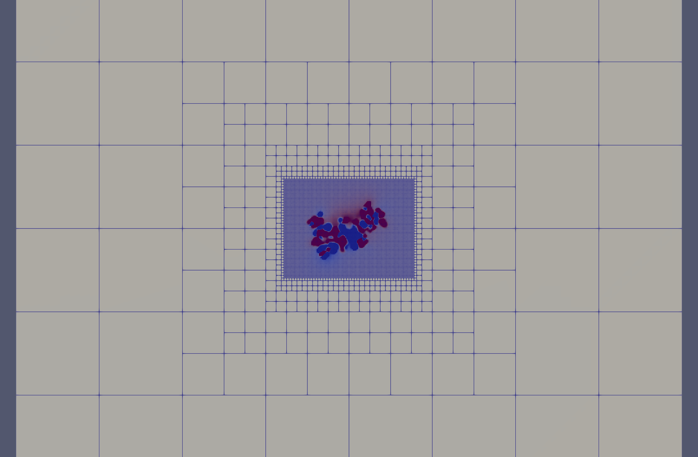
What are perfil1 and perfil2?

The perfil parameters control how the mesh adapts to the geometry of the molecule by defining how densely the mesh is refined in different regions of the domain. Specifically, they represent filling percentages:

• perfil1 is the ratio between the molecular system size and the edge length of the finest resolution region (core mesh).
• perfil2 is the same ratio, but for the outer region where the mesh is coarser.

This means:

• A higher value of perfil1 leads to finer elements near the molecule.
• A lower perfil2 defines coarser elements at the domain boundary.

The mesh gradually transitions from the fine region (perfil1) to the coarse one (perfil2), allowing accurate resolution where needed while keeping the overall number of elements manageable.

---

Step 2 – Run the Solver

Now launch the simulation using Apptainer:

apptainer exec --pwd /App --bind .:/App ../NextGenPB.sif mpirun -np 4 ngpb --prmfile options.prm

---

Step 3 – Output and Results

At the end of the execution, you will see a log similar to this:

================ [ Electrostatic Energy ] =================
  Net charge [e]:                                 7.327471962526033e-15
  Flux charge [e]:                                -4.859124220152702e-11
  Polarization energy [kT]:                       -384.6169807703798
  Direct ionic energy [kT]:                       -0.2516508616874018
  Coulombic energy [kT]:                          -10097.24155852403
  Sum of electrostatic energy contributions [kT]: -10482.11019015609
===========================================================
compute energy
Elapsed time : 141.198ms

Timing Report:
...

This includes the timing report and the electrostatic energy of the system. These outputs confirm that NextGenPB is functioning correctly and that your configuration is valid.

---

➡️ Go to the next exercise.