Exercise Three: Outputs
In this exercise, we will learn how to generate and visualize the output files produced by NextGenPB.
Step 1 – Prepare the Inputs
Go to the directory for the third exercise:
cd ~/ngpb_tutorial/ex3
This will be your working directory:
~/ngpb_tutorial/ex3
Copy a .pdb file into your current directory:
cp ../NextGenPB/data/1CCM.pdb .
.pdb files do not contain partial charges or atomic radii, which are necessary to compute the molecular surface and electrostatics. These data are included in .pqr files.
So you must also copy the files that provide this information:
cp ../NextGenPB/data/charge.crg .
cp ../NextGenPB/data/radius.siz .
Prepare the Parameter File
Create a file named options.prm in the current directory with the following content:
[input]
filetype = pdb
filename = 1CCM.pdb
radius_file = radius.siz
charge_file = charge.crg
write_pqr = 1
name_pqr = 1CCM_out.pqr
[../]

[mesh]
mesh_shape = 0
perfil1 = 0.95
perfil2 = 0.2
scale   = 2.0
[../]

[model]
bc_type = 1
molecular_dielectric_constant = 2      # Dielectric constant inside the molecule
solvent_dielectric_constant   = 80     # Dielectric constant of the solvent (e.g., water)
ionic_strength                = 0.145  # Ionic strength (mol/L)
T                             = 298.15 # Temperature in Kelvin
calc_energy    = 2
calc_coulombic = 1

atoms_write   = 1     # 1 = write potential at atom centers, 0 = don't
map_type      = vtu   # Output format: 'vtu' (for ParaView, vtk binary), 'oct' (Octbin internal format)
potential_map = 1     # 1 = write full potential map to file
eps_map       = 1     # 1 = write dielectric (epsilon) map to file
surf_write    = 1     # 1 = write potential on the molecular surface
[../]
This configuration enables NextGenPB to generate all the available output files, including dielectric and electrostatic potential maps, surface potentials, and values at atomic positions.
Step 2 – Run the Solver
Now launch the simulation using Apptainer:
apptainer exec --pwd /App --bind .:/App ../NextGenPB.sif mpirun -np 4 ngpb --prmfile options.prm
Step 3 – Output and Results
At the end of the execution, you will see a log similar to this:
================ [ Electrostatic Energy ] =================
  Net charge [e]:                                 1.000100072473288
  Flux charge [e]:                                0.9999852578120542
  Polarization energy [kT]:                       -370.6199322776101
  Direct ionic energy [kT]:                       -0.3187630925742346
  Coulombic energy [kT]:                          -10069.09853443279
  Sum of electrostatic energy contributions [kT]: -10440.03722980297
===========================================================
compute energy
Elapsed time : 140.469ms
Write potential on the surface
Elapsed time : 169.288ms
export potential map new
Elapsed time : 43.058ms
export epsilon map new
Elapsed time : 44.231ms
File .pvtu create: total_potential_map.pvtu
File .pvtu create: total_eps_map.pvtu
...
After the execution finishes, the solver will generate a set of output files:
eps_map_000*.vtu– partial dielectric maps (one per MPI rank)potential_map_000*.vtu– partial potential maps (one per MPI rank)total_eps_map.pvtu– merged dielectric map for visualization in ParaViewtotal_potential_map.pvtu– merged potential map for visualization in ParaViewphi_surf.txt– potential values on the molecular surfacephi_nodes.txt– potential values at the molecuar surface boundary nodesphi_on_atoms.txt– potential values at atomic positions
The * in the filenames corresponds to the MPI rank number.
Step 4 – Visualize
With VMD / PyMOL / ChimeraX
If you’re interested in visualizing the electrostatic potential on the molecular surface, you can use tools like VMD, PyMOL, or ChimeraX.
These popular molecular visualization tools cannot directly read .vtu or .pvtu files.
To visualize your electrostatic potential with them, you need to convert the data into a format they support — typically the Gaussian CUBE file format.
Use the vtu2cube.py script
NextGenPB provides a Python script in the scripts/ directory that converts .vtu files into .cube format.
To run this script you need the python module
vtk.Install it with:
pip install vtkor, if you’re using Anaconda:
conda install vtk
Run the following command in your terminal:
python ../NextGenPB/scripts/vtu2cube.py 1CCM_out.pqr --scale 2
This will generate a CUBE file 1CCM_out.cube.
In general, you can copy the script
vtu2cube.pyinto your working directory,
or you can add the script’s directory to yourPATHso it can be run from anywhere:export PATH=path_to_ngpb_dir/scripts:$PATH
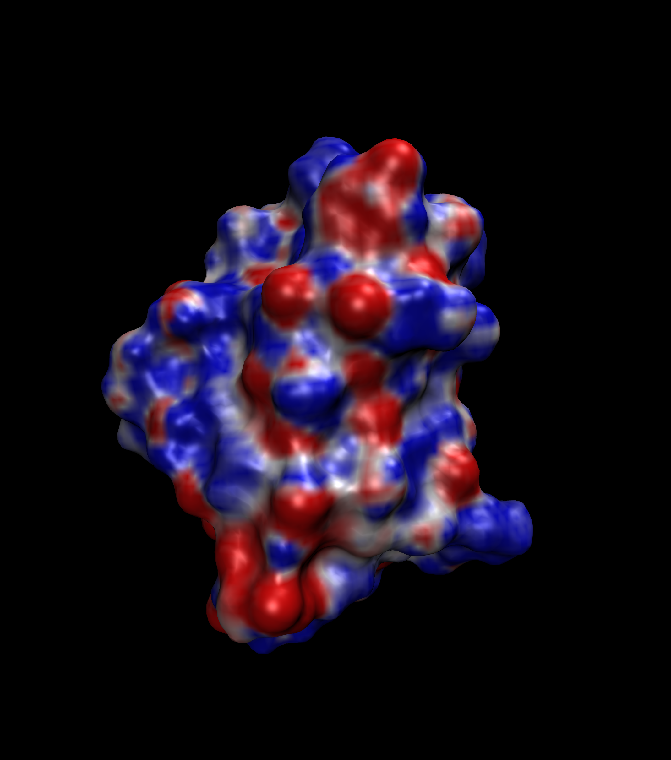
You can now load the .cube file into VMD, PyMOL, or ChimeraX to visualize the electrostatic potential mapped onto the molecular surface.
Load the .cube file in VMD, PyMOL, or ChimeraX
Now open your molecular visualization software:
- In VMD, use File > Load Data Into Molecule and select the .cube file.
- In PyMOL, use File > Open to load the .cube file.
- In ChimeraX, use the command open
1CCM_out.cube(replace filename accordingly).
These programs will display the electrostatic potential as a volumetric map or as colored surfaces mapped onto the molecule.
With ParaView
If you have ParaView or are interested in more advanced post-processing, you can use the .pvtu and .vtu files generated by the solver.
To visualize the results in ParaView:
- Open
total_potential_map.pvtuto explore the electrostatic potential field in 3D. - Use the Color Map Editor to visualize potential gradients and field distributions.
- Optionally, open
total_eps_map.pvtuto visualize dielectric interfaces and material boundaries.
For quantitative analysis, you can also import the plain-text output files such as phi_surf.txt or phi_on_atoms_*.txt into tools like Python (NumPy/Matplotlib), MATLAB, or Gnuplot.
These data files contain scalar potential values evaluated on surfaces, mesh nodes, or atomic positions, and are suitable for custom plots or further statistical processing.
➡️ Go to the next exercise.